Types of Mathematical Models
Explain the types of mathematical models and their applications in mineral processing.
Types of Mathematical Models and Their Applications in Mineral Processing
Mathematical
models in mineral processing are essential for understanding, designing, and
optimizing operations. The models are categorized based on their development
approach and the level of complexity. Below are the main types of mathematical
models and their applications:
1. Phenomenological Models
- Definition:
These models are based on fundamental physical and chemical principles, such as mass balance, energy balance, and population balance. They aim to describe the behavior of processes based on underlying mechanisms. - Applications:
- Modeling comminution processes to
predict particle size distribution.
- Understanding particle motion in
hydrocyclones.
- Analyzing flotation kinetics and
bubble-particle interactions.
2. Empirical Models
- Definition:
Empirical models rely on experimental data and observations rather than theoretical principles. They are often expressed as regression equations or correlations. - Applications:
- Estimating grinding energy
requirements using Bond’s law.
- Predicting classifier and screen
efficiency based on performance data.
- Calculating recovery and grade in
beneficiation processes.
3. Population Balance Models (PBM)
- Definition:
These models describe the size and composition changes in a population of particles as they undergo processes such as grinding or separation. - Applications:
- Modeling the breakage and
selection functions in grinding circuits.
- Simulating classification
processes in hydrocyclones and vibrating screens.
- Describing mineral liberation
during comminution.
4. Kinetic Models
- Definition:
Kinetic models describe the rates at which processes occur, such as chemical reactions or separations, and are often represented by rate equations. - Applications:
- Modeling flotation processes
based on reaction kinetics between minerals and reagents.
- Analyzing leaching rates in
hydrometallurgical processes.
- Predicting froth stability and
recovery over time in flotation circuits.
5. Statistical and Data-Driven Models
- Definition:
These models use statistical techniques or machine learning algorithms to analyze historical data and predict system behavior. - Applications:
- Predicting plant throughput based
on historical feed data.
- Optimizing process parameters
using regression models.
- Identifying trends and correlations
in process data.
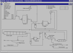
6. Simulation Models
- Definition:
Simulation models integrate multiple unit operations and simulate the overall behavior of a mineral processing plant. These models are typically used to analyze and optimize entire plant operations. - Applications:
- Designing and testing new plant
flow sheets.
- Conducting sensitivity analysis
to assess the impact of changing parameters.
- Reducing operational costs by
simulating process improvements.
7. Hybrid Models
- Definition:
Hybrid models combine phenomenological and empirical approaches to address complex processes that are difficult to model using a single method. - Applications:
- Modeling hydrocyclones using
fluid mechanics principles with empirically derived parameters.
- Simulating flotation processes by
combining kinetic and data-driven approaches.
Conclusion
The selection
of a mathematical model depends on the complexity of the process, the
availability of data, and the purpose of the study. Each type of model has its
specific applications and contributes to the understanding and optimization of
mineral processing systems, ensuring efficient and cost-effective plant
operations.
Reference: R.P. King, Modeling and Simulation
of Mineral Processing Systems, p. 3–4.
Comments
Post a Comment